Benchmarking distance choices • manydist

1 Overview

Mixed-type data do not determine a unique dissimilarity. Different choices about scaling, categorical comparisons, commensurability, and associations can produce different geometries and, consequently, different learning results.

manydist provides three helpers for studying these choices systematically:

all_dist_method_specs() constructs tables of valid specifications;
benchmark_mdist() evaluates mdist() once for every row and compares all successful distances;
benchmark_comparisons() extracts the pairwise diagnostics.

This guide shows how to define a manageable candidate set, run it safely, inspect failures, compare the resulting dissimilarities, and optionally assess their clustering solutions. The benchmark is a sensitivity-analysis tool; the final choice should still be based on the intended downstream task and an appropriate validation design.

2 Setup

library(manydist)
library(dplyr)
library(tidyr)
library(ggplot2)

We use complete cases from palmerpenguins. The species label is retained for later use, but the first benchmark is deliberately unsupervised and uses only the predictors.

penguins_small <- palmerpenguins::penguins |>
  dplyr::select(
    species,
    bill_length_mm,
    bill_depth_mm,
    flipper_length_mm,
    body_mass_g,
    island,
    sex
  ) |>
  tidyr::drop_na()

penguin_x <- penguins_small |>
  dplyr::select(-species)

dplyr::glimpse(penguin_x)

Rows: 333
Columns: 6
$ bill_length_mm    <dbl> 39.1, 39.5, 40.3, 36.7, 39.3, 38.9, 39.2, 41.1, 38.6…
$ bill_depth_mm     <dbl> 18.7, 17.4, 18.0, 19.3, 20.6, 17.8, 19.6, 17.6, 21.2…
$ flipper_length_mm <int> 181, 186, 195, 193, 190, 181, 195, 182, 191, 198, 18…
$ body_mass_g       <int> 3750, 3800, 3250, 3450, 3650, 3625, 4675, 3200, 3800…
$ island            <fct> Torgersen, Torgersen, Torgersen, Torgersen, Torgerse…
$ sex               <fct> male, female, female, female, male, female, male, fe…

3 Constructing a candidate set

all_dist_method_specs() returns one specification per row. Preset rows use the preset column, whereas component rows describe a custom combination of method_cat, method_num, and commensurable.

all_dist_method_specs(mode = "presets_only") |>
  dplyr::select(
    spec_type,
    preset,
    method_cat,
    method_num,
    commensurable
  )

# A tibble: 10 × 5
   spec_type preset    method_cat method_num commensurable
   <chr>     <chr>     <chr>      <chr>      <lgl>
 1 preset    euclidean <NA>       <NA>       NA
 2 preset    gower     <NA>       <NA>       NA
 3 preset    hl        <NA>       <NA>       NA
 4 preset    u_dep     <NA>       <NA>       NA
 5 preset    u_indep   <NA>       <NA>       NA
 6 preset    u_mix     <NA>       <NA>       NA
 7 preset    dkss      <NA>       <NA>       NA
 8 preset    gudmm     <NA>       <NA>       NA
 9 preset    mod_gower <NA>       <NA>       NA
10 preset    custom    <NA>       <NA>       NA

It is usually better to begin with a small set of substantively different choices than to run every possible combination. Here we compare four presets and two custom specifications.

candidate_specs <- dplyr::bind_rows(
  all_dist_method_specs(
    mode = "presets_only",
    preset = c("gower", "u_indep", "euclidean", "hl")
  ),
  tibble::tibble(
    spec_type = "component",
    preset = "custom",
    method_cat = "matching",
    method_num = "std",
    commensurable = c(FALSE, TRUE)
  )
) |>
  dplyr::mutate(
    label = dplyr::case_when(
      preset == "gower" ~ "Gower",
      preset == "u_indep" ~ "Unbiased independent",
      preset == "euclidean" ~ "Euclidean",
      preset == "hl" ~ "Hennig--Liao",
      commensurable ~ "Matching + z scores (weighted)",
      TRUE ~ "Matching + z scores"
    )
  )

candidate_specs

# A tibble: 6 × 6
  spec_type preset    method_cat method_num commensurable label
  <chr>     <chr>     <chr>      <chr>      <lgl>         <chr>
1 preset    euclidean <NA>       <NA>       NA            Euclidean
2 preset    gower     <NA>       <NA>       NA            Gower
3 preset    hl        <NA>       <NA>       NA            Hennig--Liao
4 preset    u_indep   <NA>       <NA>       NA            Unbiased independent
5 component custom    matching   std        FALSE         Matching + z scores
6 component custom    matching   std        TRUE          Matching + z scores (…

This explicit table is useful for reproducibility: it records exactly which distance definitions entered the comparison.

4 Running the benchmark

benchmark_mdist() applies mdist() to each specification and compares every pair of successful results. An error in one row does not stop the remaining computations. By default, cluster_k = NULL, so no clustering is performed.

distance_benchmark <- benchmark_mdist(
  x = penguin_x,
  specs = candidate_specs
)

distance_benchmark |>
  dplyr::select(
    spec_type,
    preset,
    method_cat,
    method_num,
    commensurable,
    ok,
    error
  )

# A tibble: 6 × 7
  spec_type preset    method_cat method_num commensurable ok    error
  <chr>     <chr>     <chr>      <chr>      <lgl>         <lgl> <chr>
1 preset    euclidean <NA>       <NA>       NA            TRUE  <NA>
2 preset    gower     <NA>       <NA>       NA            TRUE  <NA>
3 preset    hl        <NA>       <NA>       NA            TRUE  <NA>
4 preset    u_indep   <NA>       <NA>       NA            TRUE  <NA>
5 component custom    matching   std        FALSE         TRUE  <NA>
6 component custom    matching   std        TRUE          TRUE  <NA>

The returned MDistBenchmark object remains a tibble and adds three columns:

result contains the MDist object, or the captured error;
ok indicates whether computation succeeded;
error contains the error message for an unsuccessful row.

distance_benchmark |>
  dplyr::count(ok)

# A tibble: 1 × 2
  ok        n
  <lgl> <int>
1 TRUE      6

Failed specifications remain easy to inspect.

distance_benchmark |>
  dplyr::filter(!ok) |>
  dplyr::select(
    preset,
    method_cat,
    method_num,
    commensurable,
    error
  )

# A tibble: 0 × 5
# ℹ 5 variables: preset <chr>, method_cat <chr>, method_num <chr>,
#   commensurable <lgl>, error <chr>

This behavior is especially helpful for larger sensitivity analyses, where some methods may be incompatible with the variables in a particular data set.

5 Comparing successful distances

benchmark_comparisons() returns one row for each unique pair of successful specifications. Four diagnostics are always available:

mad is the mean absolute difference between the corresponding pairwise dissimilarities;
relative_distance divides MAD by the average magnitude of the two distances;
mds_congruence compares their classical MDS configurations;
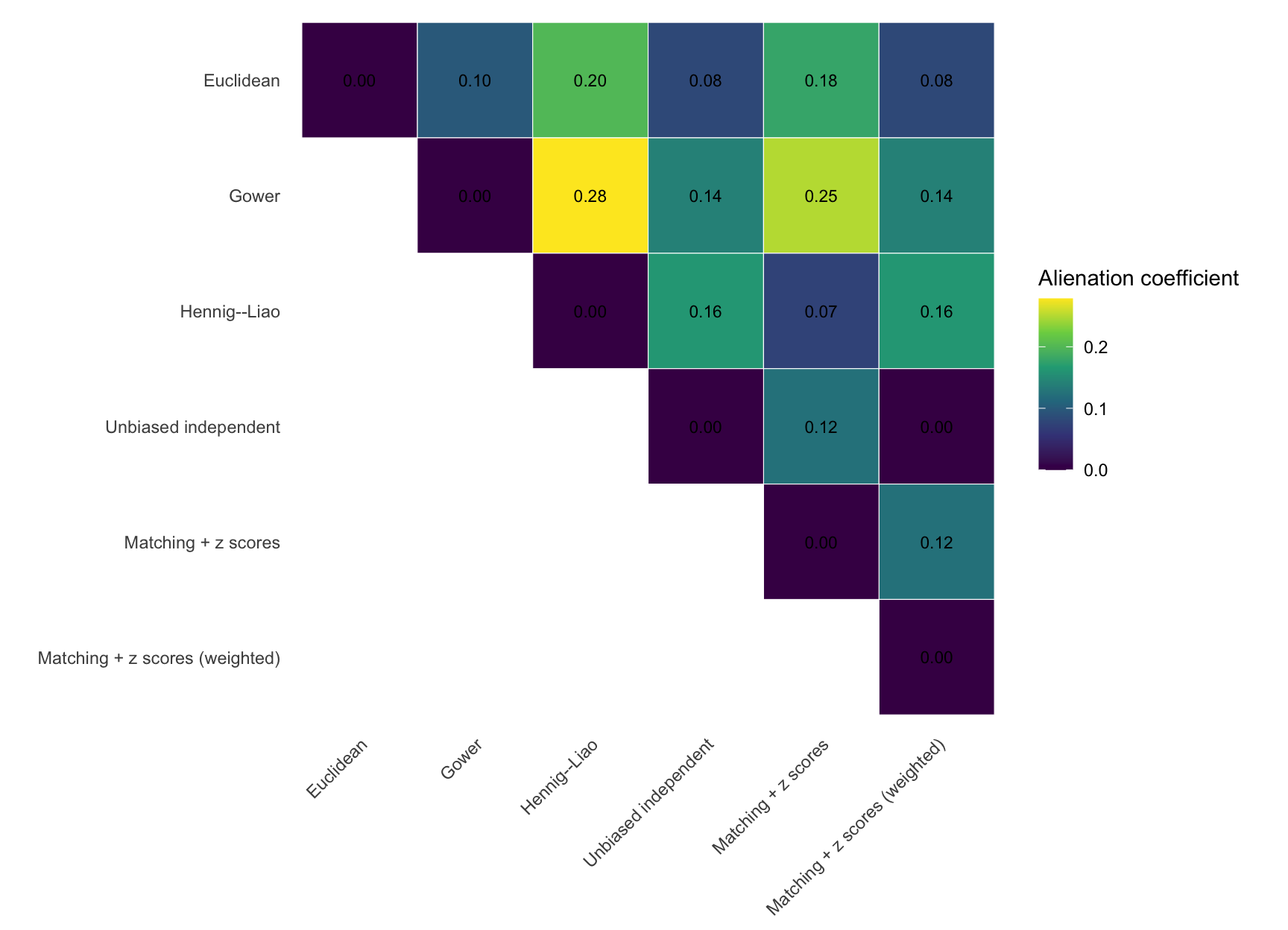
alienation is $\sqrt{1-c^2}$ , where $c$ is MDS congruence.

The symmetric relative distance is

$\frac{2\operatorname{mean}(|d_a-d_b|)} {\operatorname{mean}(|d_a|)+\operatorname{mean}(|d_b|)}.$

It is zero for identical distances and does not depend on how many specifications are included in the benchmark.

pairwise_diagnostics <- benchmark_comparisons(distance_benchmark)

pairwise_diagnostics |>
  dplyr::select(
    method_1,
    method_2,
    mad,
    relative_distance,
    mds_congruence,
    alienation
  ) |>
  dplyr::arrange(dplyr::desc(relative_distance)) |>
  dplyr::slice_head(n = 10)

# A tibble: 10 × 6
   method_1     method_2         mad relative_distance mds_congruence alienation
   <chr>        <chr>          <dbl>             <dbl>          <dbl>      <dbl>
 1 Gower        Unbiased inde…  5.66             1.78           0.990     0.141
 2 Gower        Matching + z …  5.66             1.78           0.990     0.141
 3 Gower        Matching + z …  5.33             1.76           0.968     0.250
 4 Euclidean    Gower           3.64             1.67           0.995     0.0981
 5 Gower        Hennig--Liao    2.58             1.57           0.961     0.278
 6 Hennig--Liao Unbiased inde…  3.08             0.687          0.987     0.162
 7 Hennig--Liao Matching + z …  3.08             0.687          0.987     0.162
 8 Hennig--Liao Matching + z …  2.74             0.636          0.997     0.0747
 9 Euclidean    Unbiased inde…  2.07             0.414          0.997     0.0807
10 Euclidean    Matching + z …  2.07             0.414          0.997     0.0807

Raw MAD retains differences in absolute scale. Relative distance makes those differences comparable, while congruence and alienation describe changes in the induced geometry. The measures are complementary rather than competing rankings.

autoplot() displays any diagnostic as an annotated triangular heatmap. The optional label column in candidate_specs supplies the axis labels.

Relative distance
Alienation

ggplot2::autoplot(
  distance_benchmark,
  metric = "alienation",
  digits = 2
)

Triangular heatmap of pairwise alienation coefficients among six distance specifications.

6 Optional clustering comparisons

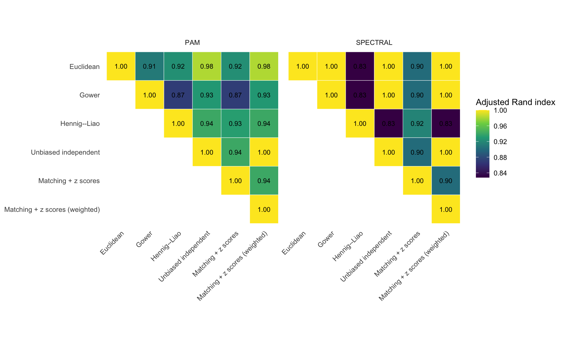
Supplying cluster_k asks the benchmark to cluster every successful distance. The same value of $K$ and the same clustering method are used within each pairwise comparison. Available methods are "pam", "hclust", and "spectral". If cluster_k is omitted or NULL, this potentially expensive step is skipped.

set.seed(2026)

clustering_benchmark <- benchmark_mdist(
  x = penguin_x,
  specs = candidate_specs,
  cluster_k = 3,
  cluster_methods = c("pam", "spectral"),
  spectral_nstart = 50
)

benchmark_comparisons(clustering_benchmark) |>
  dplyr::select(
    method_1,
    method_2,
    ari_pam,
    ari_spectral
  ) |>
  dplyr::arrange(ari_pam) |>
  dplyr::slice_head(n = 10)

# A tibble: 10 × 4
   method_1             method_2                       ari_pam ari_spectral
   <chr>                <chr>                            <dbl>        <dbl>
 1 Gower                Hennig--Liao                     0.870        0.828
 2 Gower                Matching + z scores              0.871        0.901
 3 Euclidean            Gower                            0.911        1
 4 Euclidean            Matching + z scores              0.924        0.901
 5 Euclidean            Hennig--Liao                     0.924        0.828
 6 Gower                Unbiased independent             0.929        1
 7 Gower                Matching + z scores (weighted)   0.929        1
 8 Hennig--Liao         Matching + z scores              0.933        0.917
 9 Unbiased independent Matching + z scores              0.941        0.901
10 Matching + z scores  Matching + z scores (weighted)   0.941        0.901

The adjusted Rand indices compare two unsupervised partitions; the penguin species labels are not used. An ARI of one indicates identical assignments, whereas smaller values indicate greater sensitivity to the distance specification.

ggplot2::autoplot(
  clustering_benchmark,
  metric = "ari",
  digits = 2
)

Faceted triangular heatmaps of pairwise adjusted Rand indices for PAM and spectral clustering.

7 Response-aware candidates

Some specifications can use a response when constructing the dissimilarity. They can be listed with mode = "response_aware_only".

response_specs <- all_dist_method_specs(
  mode = "response_aware_only"
) |>
  dplyr::filter(
    spec_type == "preset",
    preset %in% c("u_dep", "u_mix")
  )

response_specs

# A tibble: 2 × 5
  spec_type preset method_cat method_num commensurable
  <chr>     <chr>  <chr>      <chr>      <lgl>
1 preset    u_dep  <NA>       <NA>       NA
2 preset    u_mix  <NA>       <NA>       NA

When the response is supplied to benchmark_mdist(), it is used only by response-aware components and is not treated as an ordinary predictor.

response_benchmark <- benchmark_mdist(
  x = penguins_small,
  response = species,
  specs = response_specs
)

response_benchmark |>
  dplyr::select(preset, ok, error)

# A tibble: 2 × 3
  preset ok    error
  <chr>  <lgl> <chr>
1 u_dep  TRUE  <NA>
2 u_mix  TRUE  <NA>

benchmark_comparisons(response_benchmark)

# A tibble: 1 × 8
  method_1_id method_2_id method_1 method_2   mad relative_distance
        <int>       <int> <chr>    <chr>    <dbl>             <dbl>
1           1           2 u_dep    u_mix     1.30             0.215
# ℹ 2 more variables: mds_congruence <dbl>, alienation <dbl>

If response-aware distances are compared by predictive performance, their construction must occur inside each resample. Constructing them once from the full outcome vector would leak assessment information into training.

The recipe interface handles this separation directly. When a response-aware specification is used in step_mdist(), the step discovers the single recipe outcome and fits the response-aware profiles using only the current analysis set. The fitted profiles are then applied to assessment observations without using their outcomes. Set response_used = FALSE when the comparison should use the predictor-only form of a response-aware specification.

8 Scaling up a comparison

The same workflow can be expanded by filtering the full specification table, as in the unevaluated example below. Keep in mind that $M$ successful specifications produce $M(M-1)/2$ pairwise rows, and clustering adds one fitted partition for every distance and clustering-method combination.

larger_specs <- all_dist_method_specs(
  mode = "full",
  method_cat = c("matching", "tvd"),
  method_num = c("std", "robust"),
  commensurable = c(FALSE, TRUE)
)

larger_benchmark <- benchmark_mdist(
  x = penguins_small,
  response = species,
  specs = larger_specs
)

Before expanding the grid, decide what the benchmark is intended to measure:

for clustering, compare stability, separation, or external labels when legitimately available;
for prediction, compare candidates through resampling and preserve a final test set;
for exploratory analysis, inspect whether substantive conclusions are stable across plausible distance definitions;
always keep unsuccessful rows and their messages as part of the audit trail.

The clustering and supervised-learning guides show how MDist specifications enter those downstream workflows.