manydist: distance-based learning with mixed-type data

1 Overview

manydist provides tools for constructing dissimilarities for numerical, categorical, and mixed-type data.

The main function is mdist(). It computes a dissimilarity object that can be used in distance-based learning workflows, including clustering, nearest-neighbour prediction, and diagnostic analyses.

The package supports both preset specifications and custom specifications. In the current interface:

method_cat controls the categorical dissimilarity;
method_num controls the preprocessing of numerical variables;
commensurable controls whether variable-wise contributions are placed on a comparable scale;
preset selects a predefined distance specification.

The numerical metric is no longer a user-facing argument. For most presets, numerical variables are compared through Manhattan-type contributions. The exceptions are presets such as "hl" and "euclidean", where the Euclidean structure is part of the definition.

The "euclidean" preset replaces the former "euclidean_onehot" name. It computes Euclidean distances after one-hot encoding categorical variables.

2 Setup

library(manydist)
library(dplyr)
library(tidyr)
library(recipes)

We use the palmerpenguins data for illustration.

if (requireNamespace("palmerpenguins", quietly = TRUE)) {
  data("penguins", package = "palmerpenguins")

  penguins_small <- palmerpenguins::penguins |>
    dplyr::select(
      species,
      bill_length_mm,
      bill_depth_mm,
      flipper_length_mm,
      body_mass_g,
      island,
      sex
    ) |>
    tidyr::drop_na()
}

The data contain numerical variables, such as bill length and body mass, and categorical variables, such as island and sex.

dplyr::glimpse(penguins_small)

Rows: 333
Columns: 7
$ species           <fct> Adelie, Adelie, Adelie, Adelie, Adelie, Adelie, Adel…
$ bill_length_mm    <dbl> 39.1, 39.5, 40.3, 36.7, 39.3, 38.9, 39.2, 41.1, 38.6…
$ bill_depth_mm     <dbl> 18.7, 17.4, 18.0, 19.3, 20.6, 17.8, 19.6, 17.6, 21.2…
$ flipper_length_mm <int> 181, 186, 195, 193, 190, 181, 195, 182, 191, 198, 18…
$ body_mass_g       <int> 3750, 3800, 3250, 3450, 3650, 3625, 4675, 3200, 3800…
$ island            <fct> Torgersen, Torgersen, Torgersen, Torgersen, Torgerse…
$ sex               <fct> male, female, female, female, male, female, male, fe…

3 Computing a mixed-type dissimilarity

The simplest way to compute a mixed-type dissimilarity is to use a preset.

For example, the "gower" preset computes a Gower-type dissimilarity for mixed numerical and categorical data.

d_gower <- mdist(
  penguins_small |> dplyr::select(-species),
  preset = "gower"
)

d_gower

MDist object
  preset : gower
  number of observations : 333
  number of continuous variables   : 4
  number of categorical variables   : 2
  parameters:
    - commensurability adjustment: FALSE

The resulting object stores the dissimilarity matrix and metadata about the distance specification.

class(d_gower)

[1] "MDist" "R6"

The distance matrix can be extracted with to_dist().

as.matrix(d_gower$to_dist())[1:5, 1:5]

           1          2          3          4          5
1 0.00000000 0.21132367 0.25052445 0.24090408 0.06896389
2 0.21132367 0.00000000 0.06763994 0.09064582 0.24961473
3 0.25052445 0.06763994 0.00000000 0.06252081 0.25695739
4 0.24090408 0.09064582 0.06252081 0.00000000 0.22595173
5 0.06896389 0.24961473 0.25695739 0.22595173 0.00000000

4 Response-aware dissimilarities

Some categorical dissimilarities can use a response variable. When a response is supplied to mdist(), it is used for response-aware distance construction and is removed from the predictors.

Therefore, in the following example, species is used as the response and is not also treated as a predictor.

d_response <- mdist(
  penguins_small,
  response = species,
  preset = "u_dep"
)

d_response

MDist object
  preset : u_dep
  number of observations : 333
  number of continuous variables   : 4
  number of categorical variables   : 2
  parameters:
    - categorical method: tvd
    - numerical preprocessing: pc_scores
    - commensurability adjustment: TRUE

The same can be written by passing the response as a character string.

d_response_chr <- mdist(
  penguins_small,
  response = "species",
  preset = "u_dep"
)

d_response_chr

MDist object
  preset : u_dep
  number of observations : 333
  number of continuous variables   : 4
  number of categorical variables   : 2
  parameters:
    - categorical method: tvd
    - numerical preprocessing: pc_scores
    - commensurability adjustment: TRUE

5 Custom distance specifications

Presets are convenient, but users can also define custom specifications.

In a custom specification, method_cat controls the categorical dissimilarity and method_num controls the preprocessing applied to numerical variables.

d_custom <- mdist(
  penguins_small |> dplyr::select(-species),
  preset = "custom",
  method_cat = "matching",
  method_num = "std",
  commensurable = TRUE
)

d_custom

MDist object
  preset : custom
  number of observations : 333
  number of continuous variables   : 4
  number of categorical variables   : 2
  parameters:
    - categorical method: matching
    - numerical preprocessing: std
    - commensurability adjustment: TRUE
    - number of principal components: 6
    - inertia threshold: NULL

Here, categorical variables are compared using matching dissimilarities, numerical variables are standardized, and variable-wise contributions are made commensurable.

A response-aware custom specification can also be used.

d_custom_response <- mdist(
  penguins_small,
  response = species,
  preset = "custom",
  method_cat = "tvd",
  method_num = "std",
  commensurable = TRUE
)

d_custom_response

MDist object
  preset : custom
  number of observations : 333
  number of continuous variables   : 4
  number of categorical variables   : 2
  parameters:
    - categorical method: tvd
    - numerical preprocessing: std
    - commensurability adjustment: TRUE
    - number of principal components: 6
    - inertia threshold: NULL

If only one categorical predictor is available, methods that require more than one categorical variable may switch to a simpler alternative internally.

6 Euclidean preset

The "euclidean" preset computes Euclidean distances after converting categorical variables to one-hot dummy variables.

d_euclidean <- mdist(
  penguins_small |> dplyr::select(-species),
  preset = "euclidean"
)

d_euclidean

MDist object
  preset : euclidean
  number of observations : 333
  number of continuous variables   : 4
  number of categorical variables   : 2
  parameters:
    - numerical preprocessing: std

This preset replaces the former "euclidean_onehot" name.

7 Comparing presets

Different presets encode different assumptions about how numerical and categorical variables should contribute to the final dissimilarity.

d_u_indep <- mdist(
  penguins_small |> dplyr::select(-species),
  preset = "u_indep"
)

d_u_mix <- mdist(
  penguins_small |> dplyr::select(-species),
  preset = "u_mix"
)

d_hl <- mdist(
  penguins_small |> dplyr::select(-species),
  preset = "hl"
)

d_u_indep

MDist object
  preset : u_indep
  number of observations : 333
  number of continuous variables   : 4
  number of categorical variables   : 2
  parameters:
    - categorical method: matching
    - numerical preprocessing: std
    - commensurability adjustment: TRUE

d_u_mix

MDist object
  preset : u_mix
  number of observations : 333
  number of continuous variables   : 4
  number of categorical variables   : 2
  parameters:
    - categorical method: tvd
    - numerical preprocessing: std
    - commensurability adjustment: TRUE

d_hl

MDist object
  preset : hl
  number of observations : 333
  number of continuous variables   : 4
  number of categorical variables   : 2
  parameters:
    - categorical method: HLeucl
    - numerical preprocessing: std
    - commensurability adjustment: FALSE

The available presets include:

c(
  "custom",
  "gower",
  "euclidean",
  "unbiased_dependent",
  "u_dep",
  "u_indep",
  "u_mix",
  "hl",
  "gudmm",
  "dkss",
  "mod_gower"
)

 [1] "custom"             "gower"              "euclidean"
 [4] "unbiased_dependent" "u_dep"              "u_indep"
 [7] "u_mix"              "hl"                 "gudmm"
[10] "dkss"               "mod_gower"

Some presets are intended mainly for train-train dissimilarities and may not support distances from new observations to training observations.

8 Distances from new observations to training observations

mdist() can also compute distances from new observations to the training observations through the new_data argument.

set.seed(123)

split_id <- sample(seq_len(nrow(penguins_small)), size = floor(0.75 * nrow(penguins_small)))

penguins_train <- penguins_small[split_id, ]
penguins_test  <- penguins_small[-split_id, ]

d_new <- mdist(
  x = penguins_train |> dplyr::select(-species),
  new_data = penguins_test |> dplyr::select(-species),
  preset = "gower"
)

d_new

MDist object
  preset : gower
  number of training observations : 249
  number of test observations     : 84
  number of continuous variables   : 4
  number of categorical variables   : 2
  parameters:
    - commensurability adjustment: FALSE

The resulting dissimilarity is rectangular: rows correspond to test observations and columns correspond to training observations.

dim(as.matrix(d_new$distance))

[1]  84 249

9 Using `manydist` in recipe workflows

The function step_mdist() provides a recipe interface to mdist(). It replaces selected predictors with a distance-based representation.

In supervised workflows, the response is defined on the left-hand side of the recipe formula. Therefore, when we select recipes::all_predictors(), the response variable is not used as a predictor in the distance computation.

rec <- recipes::recipe(species ~ ., data = penguins_small) |>
  step_mdist(
    recipes::all_predictors(),
    preset = "gower",
    output = "distance_to_training"
  )

rec_prep <- recipes::prep(rec, training = penguins_small)

baked <- recipes::bake(rec_prep, new_data = penguins_small)

baked |>
  dplyr::slice_head(n = 5)

# A tibble: 5 × 334
  species dist_1 dist_2 dist_3 dist_4 dist_5 dist_6 dist_7 dist_8 dist_9 dist_10
  <fct>    <dbl>  <dbl>  <dbl>  <dbl>  <dbl>  <dbl>  <dbl>  <dbl>  <dbl>   <dbl>
1 Adelie  0      0.211  0.251  0.241  0.0690 0.192  0.101  0.229  0.0832  0.153
2 Adelie  0.211  0      0.0676 0.0906 0.250  0.0338 0.278  0.0527 0.262   0.331
3 Adelie  0.251  0.0676 0      0.0625 0.257  0.0694 0.271  0.0518 0.277   0.324
4 Adelie  0.241  0.0906 0.0625 0      0.226  0.0851 0.250  0.103  0.238   0.273
5 Adelie  0.0690 0.250  0.257  0.226  0      0.251  0.0820 0.281  0.0259  0.0957
# ℹ 323 more variables: dist_11 <dbl>, dist_12 <dbl>, dist_13 <dbl>,
#   dist_14 <dbl>, dist_15 <dbl>, dist_16 <dbl>, dist_17 <dbl>, dist_18 <dbl>,
#   dist_19 <dbl>, dist_20 <dbl>, dist_21 <dbl>, dist_22 <dbl>, dist_23 <dbl>,
#   dist_24 <dbl>, dist_25 <dbl>, dist_26 <dbl>, dist_27 <dbl>, dist_28 <dbl>,
#   dist_29 <dbl>, dist_30 <dbl>, dist_31 <dbl>, dist_32 <dbl>, dist_33 <dbl>,
#   dist_34 <dbl>, dist_35 <dbl>, dist_36 <dbl>, dist_37 <dbl>, dist_38 <dbl>,
#   dist_39 <dbl>, dist_40 <dbl>, dist_41 <dbl>, dist_42 <dbl>, …

The resulting data contain the outcome variable, species, together with one distance column for each training observation. These columns are named dist_1, dist_2, and so on.

10 Custom specifications in recipes

The same interface can be used with a custom distance specification.

rec_custom <- recipes::recipe(species ~ ., data = penguins_small) |>
  step_mdist(
    recipes::all_predictors(),
    preset = "custom",
    method_cat = "matching",
    method_num = "std",
    commensurable = TRUE,
    output = "distance_to_training"
  )

rec_custom_prep <- recipes::prep(rec_custom, training = penguins_small)

baked_custom <- recipes::bake(rec_custom_prep, new_data = penguins_small)

baked_custom |>
  dplyr::slice_head(n = 5)

# A tibble: 5 × 334
  species dist_1 dist_2 dist_3 dist_4 dist_5 dist_6 dist_7 dist_8 dist_9 dist_10
  <fct>    <dbl>  <dbl>  <dbl>  <dbl>  <dbl>  <dbl>  <dbl>  <dbl>  <dbl>   <dbl>
1 Adelie    0      3.01   3.93   3.73   1.55  2.57    2.31   3.47  1.87     3.56
2 Adelie    3.01   0      1.56   2.11   3.87  0.779   4.55   1.25  4.14     5.84
3 Adelie    3.93   1.56   0      1.50   4.07  1.60    4.45   1.18  4.55     5.73
4 Adelie    3.73   2.11   1.50   0      3.40  1.96    4.00   2.42  3.66     4.49
5 Adelie    1.55   3.87   4.07   3.40   0     3.90    1.90   4.61  0.605    2.30
# ℹ 323 more variables: dist_11 <dbl>, dist_12 <dbl>, dist_13 <dbl>,
#   dist_14 <dbl>, dist_15 <dbl>, dist_16 <dbl>, dist_17 <dbl>, dist_18 <dbl>,
#   dist_19 <dbl>, dist_20 <dbl>, dist_21 <dbl>, dist_22 <dbl>, dist_23 <dbl>,
#   dist_24 <dbl>, dist_25 <dbl>, dist_26 <dbl>, dist_27 <dbl>, dist_28 <dbl>,
#   dist_29 <dbl>, dist_30 <dbl>, dist_31 <dbl>, dist_32 <dbl>, dist_33 <dbl>,
#   dist_34 <dbl>, dist_35 <dbl>, dist_36 <dbl>, dist_37 <dbl>, dist_38 <dbl>,
#   dist_39 <dbl>, dist_40 <dbl>, dist_41 <dbl>, dist_42 <dbl>, …

In this example, method_cat = "matching" specifies the categorical dissimilarity, while method_num = "std" specifies standardization of numerical variables.

11 Pairwise dissimilarities in recipes

For distance-based clustering workflows, step_mdist() can return the within-training pairwise dissimilarity matrix by setting output = "pairwise".

In this case, the recipe is intended for training-only workflows.

penguins_predictors <- penguins_small |>
  dplyr::select(-species)

rec_pairwise <- recipes::recipe(~ ., data = penguins_predictors) |>
  step_mdist(
    recipes::all_predictors(),
    preset = "gower",
    output = "pairwise"
  )

rec_pairwise_prep <- recipes::prep(rec_pairwise, training = penguins_predictors)

pairwise_dist <- recipes::bake(
  rec_pairwise_prep,
  new_data = penguins_predictors
)

pairwise_dist |>
  dplyr::slice_head(n = 5)

# A tibble: 5 × 333
  dist_1 dist_2 dist_3 dist_4 dist_5 dist_6 dist_7 dist_8 dist_9 dist_10 dist_11
   <dbl>  <dbl>  <dbl>  <dbl>  <dbl>  <dbl>  <dbl>  <dbl>  <dbl>   <dbl>   <dbl>
1 0      0.211  0.251  0.241  0.0690 0.192  0.101  0.229  0.0832  0.153   0.213
2 0.211  0      0.0676 0.0906 0.250  0.0338 0.278  0.0527 0.262   0.331   0.0330
3 0.251  0.0676 0      0.0625 0.257  0.0694 0.271  0.0518 0.277   0.324   0.0755
4 0.241  0.0906 0.0625 0      0.226  0.0851 0.250  0.103  0.238   0.273   0.0645
5 0.0690 0.250  0.257  0.226  0      0.251  0.0820 0.281  0.0259  0.0957  0.255
# ℹ 322 more variables: dist_12 <dbl>, dist_13 <dbl>, dist_14 <dbl>,
#   dist_15 <dbl>, dist_16 <dbl>, dist_17 <dbl>, dist_18 <dbl>, dist_19 <dbl>,
#   dist_20 <dbl>, dist_21 <dbl>, dist_22 <dbl>, dist_23 <dbl>, dist_24 <dbl>,
#   dist_25 <dbl>, dist_26 <dbl>, dist_27 <dbl>, dist_28 <dbl>, dist_29 <dbl>,
#   dist_30 <dbl>, dist_31 <dbl>, dist_32 <dbl>, dist_33 <dbl>, dist_34 <dbl>,
#   dist_35 <dbl>, dist_36 <dbl>, dist_37 <dbl>, dist_38 <dbl>, dist_39 <dbl>,
#   dist_40 <dbl>, dist_41 <dbl>, dist_42 <dbl>, dist_43 <dbl>, …

12 Euclidean distances in recipes

The "euclidean" preset can also be used inside a recipe. Categorical predictors are one-hot encoded internally before the Euclidean distance is computed.

rec_euclidean <- recipes::recipe(species ~ ., data = penguins_small) |>
  step_mdist(
    recipes::all_predictors(),
    preset = "euclidean",
    output = "distance_to_training"
  )

rec_euclidean_prep <- recipes::prep(rec_euclidean, training = penguins_small)

baked_euclidean <- recipes::bake(rec_euclidean_prep, new_data = penguins_small)

baked_euclidean |>
  dplyr::slice_head(n = 5)

# A tibble: 5 × 334
  species dist_1 dist_2 dist_3 dist_4 dist_5 dist_6 dist_7 dist_8 dist_9 dist_10
  <fct>    <dbl>  <dbl>  <dbl>  <dbl>  <dbl>  <dbl>  <dbl>  <dbl>  <dbl>   <dbl>
1 Adelie    0     2.92   3.09   3.02    1.17  2.87    1.59  2.98   1.46     2.07
2 Adelie    2.92  0      0.997  1.28    3.28  0.477   3.29  0.856  3.44     3.69
3 Adelie    3.09  0.997  0      0.975   3.18  1.14    3.44  0.963  3.36     3.69
4 Adelie    3.02  1.28   0.975  0       2.96  1.23    3.25  1.45   3.04     3.24
5 Adelie    1.17  3.28   3.18   2.96    0     3.23    1.42  3.32   0.386    1.41
# ℹ 323 more variables: dist_11 <dbl>, dist_12 <dbl>, dist_13 <dbl>,
#   dist_14 <dbl>, dist_15 <dbl>, dist_16 <dbl>, dist_17 <dbl>, dist_18 <dbl>,
#   dist_19 <dbl>, dist_20 <dbl>, dist_21 <dbl>, dist_22 <dbl>, dist_23 <dbl>,
#   dist_24 <dbl>, dist_25 <dbl>, dist_26 <dbl>, dist_27 <dbl>, dist_28 <dbl>,
#   dist_29 <dbl>, dist_30 <dbl>, dist_31 <dbl>, dist_32 <dbl>, dist_33 <dbl>,
#   dist_34 <dbl>, dist_35 <dbl>, dist_36 <dbl>, dist_37 <dbl>, dist_38 <dbl>,
#   dist_39 <dbl>, dist_40 <dbl>, dist_41 <dbl>, dist_42 <dbl>, …

13 Distance-based nearest-neighbour prediction

The distance representation produced by step_mdist() can be used in downstream supervised learning workflows.

Here we illustrate a nearest-neighbour classifier using the distance-to-training representation. The recipe first converts the original mixed-type predictors into distances from each observation to the training observations. The model is then tuned over the number of neighbours.

library(tidymodels)

set.seed(123)

penguin_split <- rsample::initial_split(
  penguins_small,
  prop = 0.75,
  strata = species
)

penguin_train <- rsample::training(penguin_split)
penguin_test  <- rsample::testing(penguin_split)

set.seed(123)

penguin_folds <- rsample::vfold_cv(
  penguin_train,
  v = 5,
  strata = species
)

rec_knn <- recipes::recipe(species ~ ., data = penguin_train) |>
  step_mdist(
    recipes::all_predictors(),
    preset = "gower",
    output = "distance_to_training"
  )

knn_spec <- nearest_neighbor_dist(
  neighbors = tune::tune()
) |>
  parsnip::set_mode("classification")

knn_wf <- workflows::workflow() |>
  workflows::add_recipe(rec_knn) |>
  workflows::add_model(knn_spec)

knn_grid <- tibble::tibble(
  neighbors = c(1, 3, 5, 7, 9)
)

set.seed(123)

knn_res <- tune::tune_grid(
  knn_wf,
  resamples = penguin_folds,
  grid = knn_grid,
  metrics = yardstick::metric_set(accuracy)
)

knn_res |>
  tune::collect_metrics()

# A tibble: 5 × 7
  neighbors .metric  .estimator  mean     n std_err .config
      <dbl> <chr>    <chr>      <dbl> <int>   <dbl> <chr>
1         1 accuracy multiclass 0.996     5 0.00392 pre0_mod1_post0
2         3 accuracy multiclass 1         5 0       pre0_mod2_post0
3         5 accuracy multiclass 0.992     5 0.00485 pre0_mod3_post0
4         7 accuracy multiclass 0.992     5 0.00485 pre0_mod4_post0
5         9 accuracy multiclass 0.988     5 0.00798 pre0_mod5_post0

best_knn <- knn_res |>
  tune::select_best(metric = "accuracy")

best_knn

# A tibble: 1 × 2
  neighbors .config
      <dbl> <chr>
1         3 pre0_mod2_post0

final_knn_wf <- knn_wf |>
  tune::finalize_workflow(best_knn)

final_knn_fit <- final_knn_wf |>
  parsnip::fit(data = penguin_train)

knn_pred <- predict(final_knn_fit, new_data = penguin_test) |>
  dplyr::bind_cols(penguin_test |> dplyr::select(species))

yardstick::accuracy(knn_pred, truth = species, estimate = .pred_class)

# A tibble: 1 × 3
  .metric  .estimator .estimate
  <chr>    <chr>          <dbl>
1 accuracy multiclass     0.988

This example uses preset = "gower", but the same workflow can be used with any mdist() preset or with a custom specification based on method_cat, method_num, and commensurable.

14 Distance-based PAM clustering

The same dissimilarities can be used for clustering. For clustering workflows, step_mdist() can return the within-training pairwise dissimilarity matrix by setting output = "pairwise".

penguins_predictors <- penguins_small |>
  dplyr::select(-species)

rec_pam <- recipes::recipe(~ ., data = penguins_predictors) |>
  step_mdist(
    recipes::all_predictors(),
    preset = "gower",
    output = "pairwise"
  )

pam_spec <- pam_dist(
  num_clusters = 3
)

pam_fit <- generics::fit(
  pam_spec,
  recipe = rec_pam,
  data = penguins_predictors
)

pam_pred <- predict(pam_fit)

pam_pred |>
  dplyr::slice_head(n = 10)

# A tibble: 10 × 1
   .pred_cluster
   <fct>
 1 1
 2 2
 3 2
 4 2
 5 1
 6 2
 7 1
 8 2
 9 1
10 1

Since the true species labels are available in this example, we can inspect the relationship between the PAM clusters and the species labels.

pam_pred |>
  dplyr::bind_cols(penguins_small |> dplyr::select(species)) |>
  dplyr::count(.pred_cluster, species)

# A tibble: 6 × 3
  .pred_cluster species       n
  <fct>         <fct>     <int>
1 1             Adelie       65
2 1             Chinstrap    34
3 2             Adelie       73
4 2             Chinstrap    34
5 3             Adelie        8
6 3             Gentoo      119

15 Distance-based spectral clustering

Spectral clustering can be used in the same way, by combining a pairwise distance recipe with the corresponding model specification.

rec_spectral <- recipes::recipe(~ ., data = penguins_predictors) |>
  step_mdist(
    recipes::all_predictors(),
    preset = "gower",
    output = "pairwise"
  )

spectral_spec <- spectral_dist(
  num_clusters = 3
)

spectral_fit <- generics::fit(
  spectral_spec,
  recipe = rec_spectral,
  data = penguins_predictors
)

spectral_pred <- predict(spectral_fit)

spectral_pred |>
  dplyr::slice_head(n = 10)

# A tibble: 10 × 1
   .pred_cluster
   <fct>
 1 2
 2 1
 3 1
 4 1
 5 2
 6 1
 7 2
 8 1
 9 2
10 2

Again, because this is an illustrative labelled data set, we can compare the resulting clusters with the observed species labels.

spectral_pred |>
  dplyr::bind_cols(penguins_small |> dplyr::select(species)) |>
  dplyr::count(.pred_cluster, species)

# A tibble: 5 × 3
  .pred_cluster species       n
  <fct>         <fct>     <int>
1 1             Adelie       73
2 1             Chinstrap    34
3 2             Adelie       73
4 2             Chinstrap    34
5 3             Gentoo      119

16 A small benchmark example

The function benchmark_mdist() applies mdist() repeatedly over a grid of distance specifications. This is useful for comparing alternative presets and custom specifications in a systematic way.

For a small example, we restrict the grid to a few specifications.

small_specs <- dplyr::bind_rows(
  all_dist_method_specs(mode = "presets_only") |>
    dplyr::filter(preset %in% c("gower", "u_dep", "u_indep", "euclidean")),

  all_dist_method_specs(
    mode = "full",
    method_cat = c("matching", "tvd"),
    method_num = c("std", "robust"),
    commensurable = c(TRUE, FALSE)
  ) |>
    dplyr::filter(spec_type == "component")
)

small_specs

# A tibble: 12 × 5
   spec_type preset    method_cat method_num commensurable
   <chr>     <chr>     <chr>      <chr>      <lgl>
 1 preset    euclidean <NA>       <NA>       NA
 2 preset    gower     <NA>       <NA>       NA
 3 preset    u_dep     <NA>       <NA>       NA
 4 preset    u_indep   <NA>       <NA>       NA
 5 component custom    matching   robust     FALSE
 6 component custom    matching   robust     TRUE
 7 component custom    matching   std        FALSE
 8 component custom    matching   std        TRUE
 9 component custom    tvd        robust     FALSE
10 component custom    tvd        robust     TRUE
11 component custom    tvd        std        FALSE
12 component custom    tvd        std        TRUE

bench_small <- benchmark_mdist(
  penguins_small,
  response = species,
  specs = small_specs
)

bench_small |>
  dplyr::select(
    spec_type,
    preset,
    method_cat,
    method_num,
    commensurable,
    ok,
    error
  )

# A tibble: 12 × 7
   spec_type preset    method_cat method_num commensurable ok    error
   <chr>     <chr>     <chr>      <chr>      <lgl>         <lgl> <chr>
 1 preset    euclidean <NA>       <NA>       NA            TRUE  <NA>
 2 preset    gower     <NA>       <NA>       NA            TRUE  <NA>
 3 preset    u_dep     <NA>       <NA>       NA            TRUE  <NA>
 4 preset    u_indep   <NA>       <NA>       NA            TRUE  <NA>
 5 component custom    matching   robust     FALSE         TRUE  <NA>
 6 component custom    matching   robust     TRUE          TRUE  <NA>
 7 component custom    matching   std        FALSE         TRUE  <NA>
 8 component custom    matching   std        TRUE          TRUE  <NA>
 9 component custom    tvd        robust     FALSE         TRUE  <NA>
10 component custom    tvd        robust     TRUE          TRUE  <NA>
11 component custom    tvd        std        FALSE         TRUE  <NA>
12 component custom    tvd        std        TRUE          TRUE  <NA>

The ok column reports whether the distance computation completed successfully. Failed specifications are kept in the output, with the corresponding error message stored in error.

bench_small |>
  dplyr::count(ok)

# A tibble: 1 × 2
  ok        n
  <lgl> <int>
1 TRUE     12

When all specifications are successful, the resulting MDist objects are stored in the result list-column and can be inspected or reused.

bench_small |>
  dplyr::filter(ok) |>
  dplyr::select(spec_type, preset, method_cat, method_num, commensurable, result) |>
  dplyr::slice_head(n = 3)

# A tibble: 3 × 6
  spec_type preset    method_cat method_num commensurable result
  <chr>     <chr>     <chr>      <chr>      <lgl>         <list>
1 preset    euclidean <NA>       <NA>       NA            <MDist>
2 preset    gower     <NA>       <NA>       NA            <MDist>
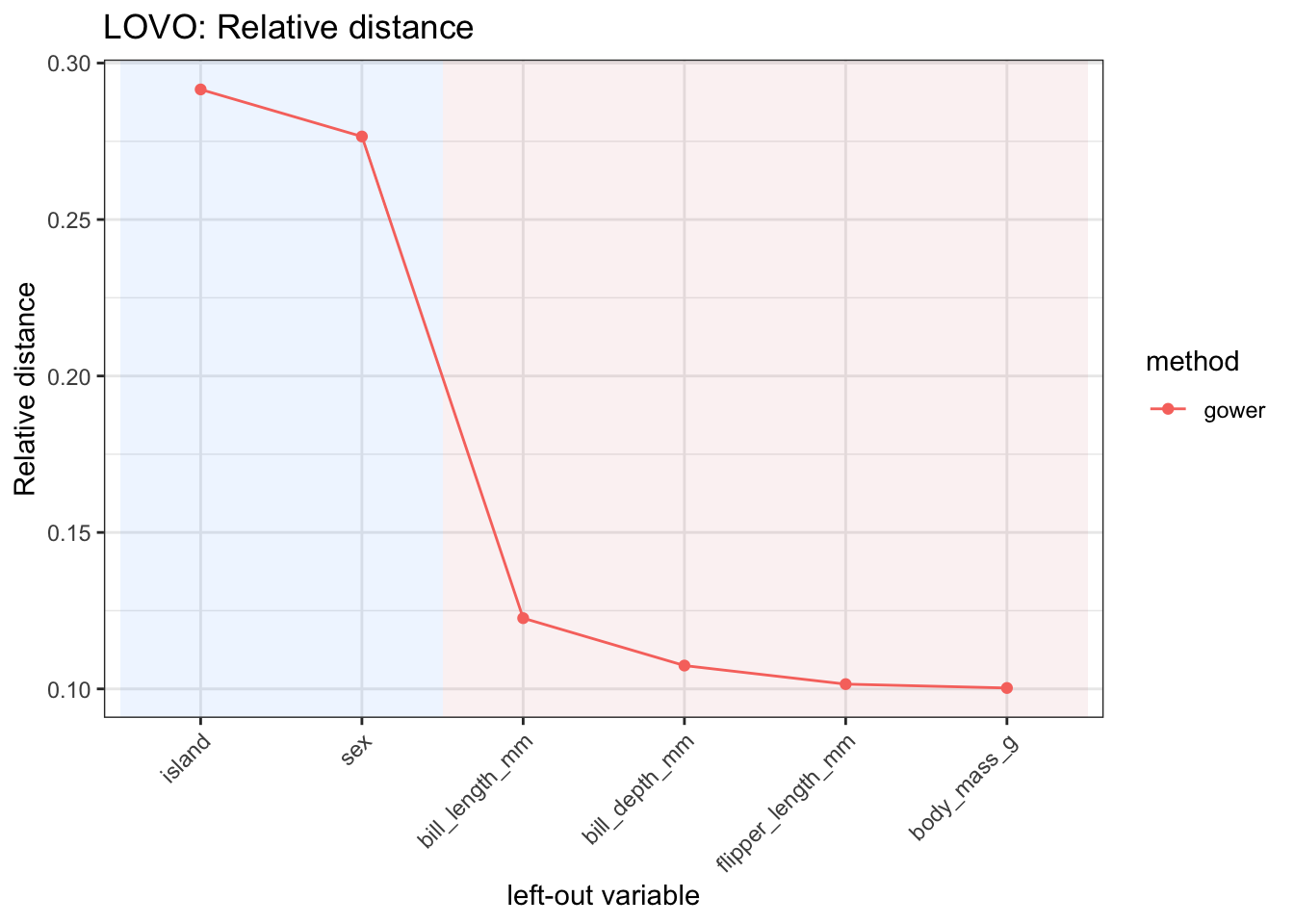
3 preset    u_dep     <NA>       <NA>       NA            <MDist>

17 Leave-one-variable-out diagnostics

lovo_mdist() computes leave-one-variable-out diagnostics for distance-based variable importance.

It first computes the full dissimilarity matrix. Then it removes one predictor at a time, recomputes the dissimilarity matrix, and compares the reduced matrix with the full one.

lovo_gower <- lovo_mdist(
  penguins_small,
  response = species,
  response_used = FALSE,
  preset = "gower"
)

lovo_gower

MDistLOVO object
  preset : gower
  dims   : 2
  n_obs  : 333
  response used : FALSE
  top vars:
# A tibble: 5 × 4
  variable          variable_type relative_distance mad_importance
  <chr>             <chr>                     <dbl>          <dbl>
1 island            categorical               0.292         0.0853
2 sex               categorical               0.277         0.0809
3 bill_length_mm    numeric                   0.123         0.0359
4 bill_depth_mm     numeric                   0.107         0.0314
5 flipper_length_mm numeric                   0.102         0.0297

The result can be summarized.

summary(lovo_gower)

Summary of MDistLOVO
  preset : gower
  dims   : 2
  n_obs  : 333
  response used : FALSE

Relative distance:
  range [0.1003, 0.2916], mean 0.1667

Top by relative distance:
# A tibble: 5 × 3
  variable          variable_type relative_distance
  <chr>             <chr>                     <dbl>
1 island            categorical               0.292
2 sex               categorical               0.277
3 bill_length_mm    numeric                   0.123
4 bill_depth_mm     numeric                   0.107
5 flipper_length_mm numeric                   0.102

The relative contribution of each variable can be visualized with autoplot().

lovo_gower$autoplot(
  metric = "relative_distance",
  reorder = TRUE
)

When response_used = FALSE, the response column is removed before computing distances. When response_used = TRUE, the response can be used by response-aware distance specifications, but it is still not treated as a predictor in the leave-one-variable-out loop.

lovo_response <- lovo_mdist(
  penguins_small,
  response = species,
  response_used = TRUE,
  preset = "u_dep"
)

lovo_response

MDistLOVO object
  preset : u_dep
  dims   : 2
  n_obs  : 333
  response used : TRUE
  top vars:
# A tibble: 5 × 4
  variable          variable_type relative_distance mad_importance
  <chr>             <chr>                     <dbl>          <dbl>
1 sex               categorical               0.171           1.04
2 bill_length_mm    numeric                   0.166           1.01
3 bill_depth_mm     numeric                   0.166           1.00
4 body_mass_g       numeric                   0.166           1.00
5 flipper_length_mm numeric                   0.166           1.00

18 Inspecting method specifications

all_dist_method_specs() returns a table of distance specifications that can be used for benchmarking or sensitivity analysis.

specs <- all_dist_method_specs()

specs |>
  dplyr::select(
    spec_type,
    preset,
    method_cat,
    method_num,
    commensurable
  ) |>
  dplyr::slice_head(n = 10)

# A tibble: 10 × 5
   spec_type preset    method_cat method_num commensurable
   <chr>     <chr>     <chr>      <chr>      <lgl>
 1 preset    euclidean <NA>       <NA>       NA
 2 preset    gower     <NA>       <NA>       NA
 3 preset    hl        <NA>       <NA>       NA
 4 preset    u_dep     <NA>       <NA>       NA
 5 preset    u_indep   <NA>       <NA>       NA
 6 preset    u_mix     <NA>       <NA>       NA
 7 preset    dkss      <NA>       <NA>       NA
 8 preset    gudmm     <NA>       <NA>       NA
 9 preset    mod_gower <NA>       <NA>       NA
10 preset    custom    <NA>       <NA>       NA

The same table can be passed to benchmark_mdist().

bench <- benchmark_mdist(
  penguins_small,
  response = species,
  specs = specs
)

bench |>
  dplyr::select(
    spec_type,
    preset,
    method_cat,
    method_num,
    commensurable,
    ok,
    error
  ) |>
  dplyr::slice_head(n = 10)

# A tibble: 10 × 7
   spec_type preset    method_cat method_num commensurable ok    error
   <chr>     <chr>     <chr>      <chr>      <lgl>         <lgl> <chr>
 1 preset    euclidean <NA>       <NA>       NA            TRUE  <NA>
 2 preset    gower     <NA>       <NA>       NA            TRUE  <NA>
 3 preset    hl        <NA>       <NA>       NA            TRUE  <NA>
 4 preset    u_dep     <NA>       <NA>       NA            TRUE  <NA>
 5 preset    u_indep   <NA>       <NA>       NA            TRUE  <NA>
 6 preset    u_mix     <NA>       <NA>       NA            TRUE  <NA>
 7 preset    dkss      <NA>       <NA>       NA            TRUE  <NA>
 8 preset    gudmm     <NA>       <NA>       NA            TRUE  <NA>
 9 preset    mod_gower <NA>       <NA>       NA            TRUE  <NA>
10 preset    custom    <NA>       <NA>       NA            TRUE  <NA>